Project Overview

Project Background

A Pew Research Center report published April 6, 2010¹ linked a decline in the US birth rate to the recession of 2008. They used birth data from 25 US States for which 2008 full-year records were available. This project was intended to investigate whether the trend was generalized to all 50 States and to see if the birth rate increased after the initial drop.

Step 1 – Extracting the Data

Population projections by State for the period 1998-2002 were stored in fixed-width format text files. This was read into R data frames and stored for later use.

library(tidyverse)

iwidths <- c(2, 1, 4, 2, rep(8, 16))
cols <- c("State", "Series", "Year", "Age", "WNHM", "WNHF", "WHM", "WHF",
          "BNHM", "BNHF", "BHM", "BHF", "AINHM", "AINHF", "AIHM", "AIHF",
          "APNHM", "APNHF", "APHM", "APHF")
st50 <- state.abb

## Test with one state first
ak0105 <- read.fwf(file = "AK0105.DAT", widths = iwidths, col.names = cols)

ak2002A <- filter(ak0105, Year == 2002 & Series == "A")
ak2002Atotal <- sum(rowSums(ak2002A[,5:20]))
ak2002B <- filter(ak0105, Year == 2002 & Series == "B")
ak2002Btotal <- sum(rowSums(ak2002B[,5:20]))
ak2001A <- filter(ak0105, Year == 2001 & Series == "A")
ak2001Atotal <- sum(rowSums(ak2001A[,5:20]))
ak2001B <- filter(ak0105, Year == 2001 & Series == "B")
ak2001Btotal <- sum(rowSums(ak2001B[,5:20]))


stpops <- tibble(Year = 2001, StateCode = "AK", Series = "A",
                 Pop = ak2001Atotal)

stpops <- rbind(stpops, tibble(Year=2001, StateCode="AK", Series="B",
                               Pop=ak2001Btotal))
stpops <- rbind(stpops, tibble(Year=2002, StateCode="AK", Series="A",
                               Pop=ak2002Atotal))
stpops <- rbind(stpops, tibble(Year=2002, StateCode="AK", Series="B",
                               Pop=ak2002Btotal))

## Do the rest
for(st in st50) {
    if(st != "AK") {
        fname <- paste0(st, "0105.DAT")
        st0105 <- read.fwf(file = fname, widths = iwidths,
                           col.names = cols)
        st2002A <- filter(st0105, Year == 2002 & Series == "A")
        st2002Atotal <- sum(rowSums(st2002A[,5:20]))
        st2002B <- filter(st0105, Year == 2002 & Series == "B")
        st2002Btotal <- sum(rowSums(st2002B[,5:20]))
        st2001A <- filter(st0105, Year == 2001 & Series == "A")
        st2001Atotal <- sum(rowSums(st2001A[,5:20]))
        st2001B <- filter(st0105, Year == 2001 & Series == "B")
        st2001Btotal <- sum(rowSums(st2001B[,5:20]))
        stpops <- rbind(stpops, tibble(Year=2001, StateCode=st, Series="A",
                                       Pop=st2001Atotal),
                        tibble(Year=2001, StateCode=st, Series="B",
                               Pop=st2001Btotal),
                        tibble(Year=2002, StateCode=st, Series="A",
                               Pop=st2002Atotal),
                        tibble(Year=2002, StateCode=st, Series="B",
                               Pop=st2002Btotal))
    }
}

for(st in st50) {
    fname <- paste0(tolower(st), "9500.txt")
    st9500 <- read.fwf(file = fname, widths = iwidths,
                       col.names = cols)
    st1998A <- filter(st9500, Year == 1998 & Series == "A")
    st1998Atotal <- sum(rowSums(st1998A[,5:20]))
    st1998B <- filter(st9500, Year == 1998 & Series == "B")
    st1998Btotal <- sum(rowSums(st1998B[,5:20]))
    st1999A <- filter(st9500, Year == 1999 & Series == "A")
    st1999Atotal <- sum(rowSums(st1999A[,5:20]))
    st1999B <- filter(st9500, Year == 1999 & Series == "B")
    st1999Btotal <- sum(rowSums(st1999B[,5:20]))
    st2000A <- filter(st9500, Year == 2000 & Series == "A")
    st2000Atotal <- sum(rowSums(st2000A[,5:20]))
    st2000B <- filter(st9500, Year == 2000 & Series == "B")
    st2000Btotal <- sum(rowSums(st2000B[,5:20]))
    stpops <- rbind(stpops, tibble(Year=1998, StateCode=st, Series="A",
                                   Pop=st1998Atotal),
                    tibble(Year=1998, StateCode=st, Series="B",
                           Pop=st1998Btotal),
                    tibble(Year=1999, StateCode=st, Series="A",
                           Pop=st1999Atotal),
                    tibble(Year=1999, StateCode=st, Series="B",
                           Pop=st1999Btotal),
                    tibble(Year=2000, StateCode=st, Series="A",
                           Pop=st2000Atotal),
                    tibble(Year=2000, StateCode=st, Series="B",
                           Pop=st2000Btotal))
}

Births by State for the period 1998-2002 were stored in tab-delimited text files. Births, total population, and crude birth rate (births per 1,000 people) by State for the period 2003-2015 were stored in tab-delimited text files. This data was read into R data frames and stored for later use.

births9502 <- read.delim(file = "1995-2002Births.txt")
births9502 <- births9502[1:408,]
births0306 <- read.delim(file = "2003-2006Births.txt", nrows = 204)
births0715 <- read.delim(file = "2007-2015Births.txt", nrows = 459)

## Select relevant columns and years from birth data
births9502 <- select(births9502, Year, State, Births) %>%
        filter(Year != 1995 & Year != 1996 & Year != 1997)
births0306 <- select(births0306, Year, State, Births, TotalPopulation, BirthRate)
births0715 <- select(births0715, Year, State, Births, TotalPopulation, BirthRate)

Step 2 – Transforming the Data

Two population projections were provided by race, Hispanic origin, and gender by single year of age for each state for each year from 1995-2005. Projection data was summed by individual projection to obtain total population by State for the years 1998-2002, and data from all States was combined into a single data frame. Data prepared this way for Alaska in 2003 was compared with the total Alaska population for 2003 in the CDC natality file for 2003-2006, and the Series B projection was a closer fit. The Series B population projections were then used for all States from 1998-2002 for subsequent analysis.

## Prepare to join based on state name in natality data
st50 <- tibble(StateCode = state.abb, State = state.name)
stpops <- inner_join(stpops, st50)

## Use Series B projections because they are closer for AK 2003
stpopsB <- filter(stpops, Series == "B")
stpopsB <- select(stpopsB, -Series)

CDC-supplied information on births by State for 1998-2002 were combined with calculated population projections for the same period, and birth rate per 1,000 total population was calculated. This time period was then combined with births and birth rate data for 2003-2015 into a single dataset. State abbreviations were added to the dataset by joining it with the built-in state dataset from R. A subset of this dataset was created by selecting data for only the 25 States whose data was used in the Pew study in order to explore potential differences in calculated birth rate over time due to selection bias.

## Join state populations and calculate birth rate (also removes DC)
births9502 <- inner_join(stpopsB, births9502) %>%
        mutate(BirthRate = Births / Pop * 1000)
names(births9502) <- c("Year", "StateCode", "TotalPopulation", "State",
                       "Births", "BirthRate")

## Put all birth data into one data frame
births <- rbind(births0306, births0715)
births <- inner_join(births, st50)
births <- births[complete.cases(births),]

births9502 <- mutate(births9502, Year = as.integer(Year)) %>%
        select(Year, State, Births, TotalPopulation, BirthRate, StateCode)
births <- rbind(births9502, births)
births <- arrange(births, Year, State)

The average US birth rate by year was obtained by summing the births and total State populations over all States and calculating the birth rate per 1,000 total population. The average birth rate by year for the 25 States whose data was used in the Pew study was obtained by summing the births and total State populations over those States and calculating the birth rate per 1,000 total population. Note that this gives “Crude Birth Rate” and not “General Fertility Rate.”

USbirths <- summarise(group_by(births, Year), sum(Births), sum(TotalPopulation))
names(USbirths) <- c("Year", "Births", "TotalPopulation")
USbirths <- mutate(USbirths, BirthRate = Births / TotalPopulation * 1000)
save(USbirths, file = "USbirths.RData")

Step 3 – Visualizing the Data

Birth rates for each State were first plotted as time series using the ggplot2 package for R and then a step-wise line showing the US average was overlaid on the base plot.

ggplot(births, aes(Year, BirthRate, color = StateCode)) + geom_point() +
        geom_step(data = USbirths, aes(x=Year, y=BirthRate, color="US",
                                        size=1), show.legend = FALSE) +
        labs(title = "Births per 1,000 People by State and US Average",
             x = "Year",
             y = "Births per 1,000 People",
             color = "State")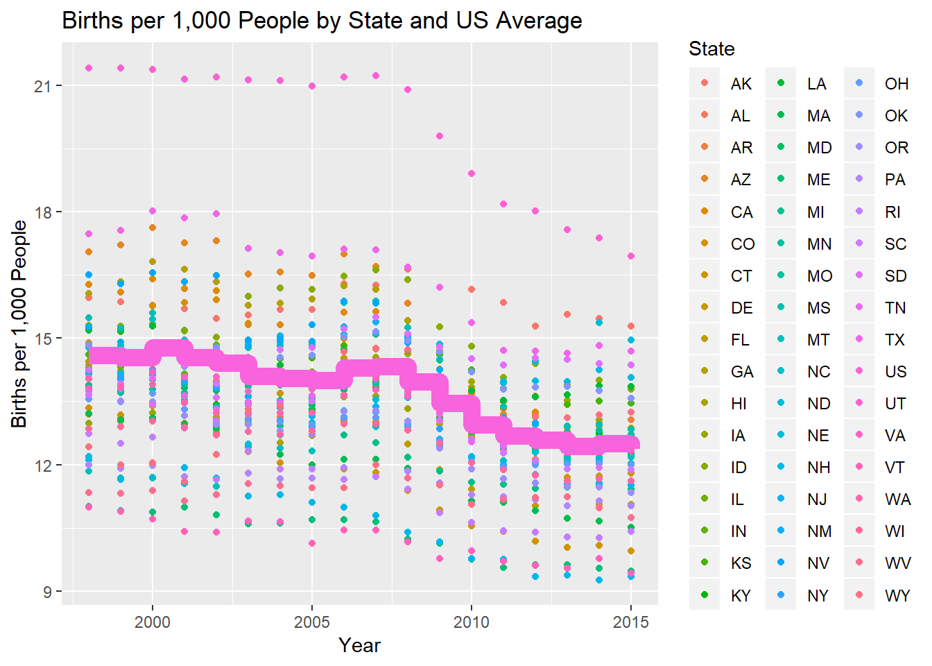

The overall US birth rate did decline sharply beginning in 2008 and has not appreciably increased since the decline began.
Average birth rate for the 25 States whose data was used in the Pew study was plotted against the average US birth rate for the same time period. The plot shows that the Pew average is consistently lower than the US average, although the differences are minor. The diagonal line shows where the points would fall if the two rates were identical.

## See if Pew states are different
pewstates <- c("AL", "AZ", "CA", "CO", "FL", "HI", "IA", "ID", "KS", "MD",
               "MI", "MN", "MO", "MS", "NC", "ND", "NE", "NH", "PA", "SD",
               "TN", "UT", "VA", "WA", "WI")
pewbirths <- filter(births, StateCode %in% pewstates)
pewsum <- summarise(group_by(pewbirths, Year), sum(Births), sum(TotalPopulation))
names(pewsum) <- c("Year", "Births", "TotalPopulation")
pewsum <- mutate(pewsum, BirthRate2 = Births / TotalPopulation * 1000)

pewplot <- tibble(Year = pewsum$Year, PewRate = pewsum$BirthRate2,
                  USRate = USbirths$BirthRate)

ggplot(data = pewplot, aes(x=USRate, y=PewRate)) + geom_point() +
        geom_abline(color = "blue", slope = 1, intercept = 0,
                    show.legend = FALSE) +
        labs(title = "Comparison of Calculated Birth Rates for 25 and 50 States",
             x = "Average Births per 1,000 People, 50 States",
             y = "Average Births per 1,000 People, 25 States\n
             (used in 2010 Pew report)")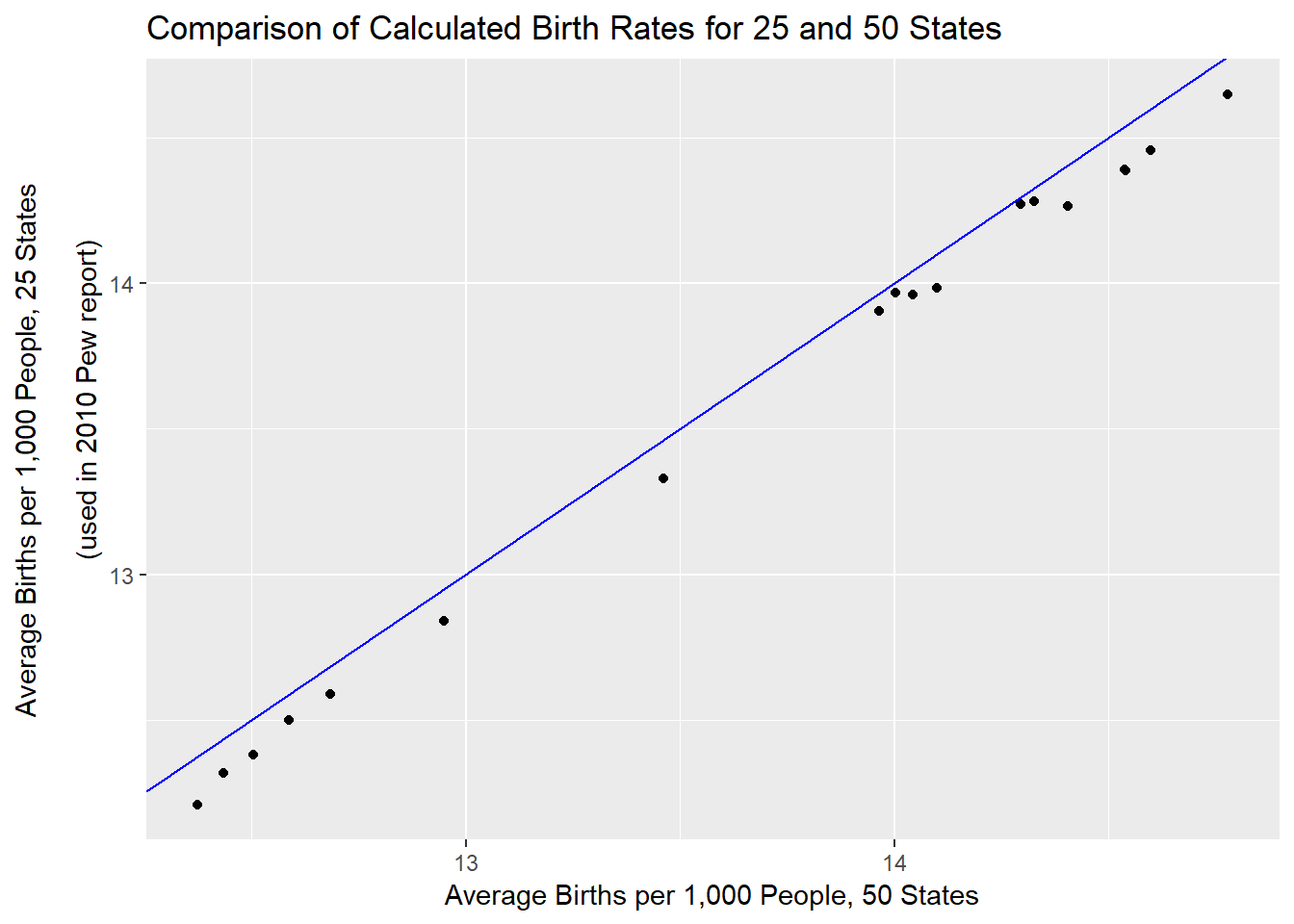

Conclusion

For the decade leading up to 2008, the US birth rate had been gradually declining. Beginning in 2008 it experienced a steep decrease, perhaps due in part to the economic circumstances. Nevertheless, the birth rate has not appreciably increased in the years since the recession, despite an improving economy.

Although the average birth rate of the 25 States whose data was used in the Pew study is somewhat lower than that calculated using data from all 50 States, the differences are small enough that the sample appears representative of the whole.